New

Choosing The Right Embedding Dimension For Semantic Search

Executive Summary: Embedding dimension — the length of the vector used to represent text, images or other data — is a critical hyperparameter for semantic search. Higher dimensions let embeddings capture finer-grained semantics, often boosting recall and precision, but come at the cost of greater latency, storage, and compute. Too few dimensions starve the model of capacity (causing underfitting), while too many invite noise or overfitting. In practice, most production search systems use moderate dimensions (e.g. 384–768) enough to cover typical content without excessive overhead. We survey recent research (e.g. DeepMind’s LIMIT theory and PCA compression studies), official docs and benchmarks, and derive practical heuristics. For example, start low (e.g. 384 dims) and measure retrieval quality increase dimensions (768, 1024, …) only if needed to close accuracy gaps. We also compare trade-offs (accuracy vs recall vs latency vs cost), cover indexing/quantization techniques (IVF/HNSW, PQ/OPQ), and list tips for training, fine-tuning, and evaluation. The bottom line: match dimension to your use case, monitor metrics, and balance accuracy gains against resource costs.

Background: What is Embedding Dimension and Why It Matters

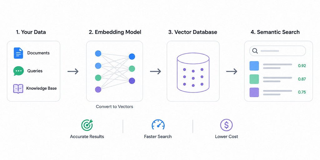
An embedding maps data (text, images, etc.) into a high-dimensional vector space, where semantic similarity corresponds to vector proximity. The dimension is simply the number of components in this vector (e.g. 384, 768, 1024, …). Think of dimension as the “resolution” or capacity of the embedding — much like image resolution: more pixels capture more detail. Higher-dimensional embeddings can encode subtler distinctions in meaning, whereas low-dimensional embeddings have limited expressivity.

Most off-the-shelf models fix the dimension a priori (e.g. BERT-base uses 768, MiniLM-v2 uses 384, CLIP uses 512, OpenAI’s text-embedding-3 uses 1536 or 2048, etc.). It is very hard to change the dimension of a pretrained model without retraining or applying post-hoc reduction. Thus, dimension selection usually happens by choosing between different models (or by dimensionality reduction of embeddings after generation).

Choosing the right dimension is a balancing act: too few dimensions will underfit your data, missing important semantic information, while too many dimensions can overfit (picking up noise or spurious correlations) and incur heavy costs. For example, one Milvus guide notes that for small datasets (only thousands of items), keeping dimension low (50–200) “prevents overfitting” and keeps the system responsive, whereas large datasets (millions of vectors) “often benefit from higher dimensions (300–1000).”

In summary, embedding dimension sets the representational capacity: it must be large enough to encode the variability in your data but not so large as to waste resources or capture noise. We now examine what research and experience tell us about this trade-off.

Theoretical Limits

Recent theory (DeepMind’s “LIMIT”) shows there are fundamental limits to what fixed-length embeddings can represent. In brief, a d-dimensional embedding can only distinguish so many combinations of documents as relevant to a query. The authors prove that for any fixed dimension, there exist query→document top‑K patterns that no embedding can encode. In practice, this means that if your application requires retrieving certain complex combinations of documents, a higher dimension may be needed (or even a different approach like multi-vector or cross-encoder retrieval). Their experiments confirm that even state-of-the-art dense retrievers fail on contrived “LIMIT” datasets when dimension is too low.

Empirical Findings

Empirical studies generally find diminishing returns beyond a few hundred dimensions. Ma et al. (2024) demonstrate that a 768-dimensional sentence-DPR embedding has most of its variance in the first ~256 components. By applying PCA, they compressed 768→256 dimensions and achieved a 48× smaller index with under 3% drop in top-100 recall. Even 96× compression was possible with modest accuracy loss. Similarly, another study found that reducing embeddings from 3072 to ~110 dimensions yielded massive speedups and memory savings with only moderate declines in ranking correlation.

In practice, vendors and benchmark papers echo that only moderate dimensions are needed for most tasks. The Milvus Quick Reference notes that a 1024‑dim vector is 4 KB (1,024×4 bytes), so 1 million vectors consume ~4 GB. It cautions that reducing dimension (e.g. 768→256) saves ~66% of space but may degrade semantic performance. Vendors recommend starting at 384 for text and 128 for images and adjusting from there.

Notably, a recent industry survey found that for most business RAG/search systems, 384–768 dimensions strike the best balance. Models with ≥1024 dims are mainly needed for specialized domains (technical, multilingual, etc.).

Benchmark Results

Major benchmarks (like HuggingFace’s MTEB) show larger models (with larger dims) often yield higher scores on varied tasks, but these gains tend to plateau. For example, a Particular blog reports that in experiments going from 768→1536 dims gave only marginal accuracy improvements. In one e-commerce test, 384‑dim embeddings already achieved 94% retrieval accuracy, while 1024‑dim gave 96% — not worth the 3× cost jump. Another example: engineers searching technical specifications resolved an ambiguity (“voltage tolerance threshold” vs “voltage threshold tolerance”) by increasing dims to 1024, illustrating a case where higher dimension captured subtle meaning differences.

Overall, the consensus is that accuracy generally increases with dimension but with rapidly diminishing returns. The trick is to find the “elbow” where adding dimensions costs more than it helps.

Trade-offs: Accuracy vs Recall vs Latency vs Cost

Choosing embedding dimension involves several trade-offs:

Accuracy/Recall: Higher dimensions can capture finer semantic details, generally improving search quality. As one blog puts it, “higher dimensions can capture more nuanced relationships between items”. However, after a point, gains shrink: many implementations see performance flattening between ~768 and 1024 dims. In fact, overly large embeddings on limited data can overfit, hurt generalization, or just redundantly encode information. The safe assumption is that if basic retrieval accuracy is already high, jumping to extreme dims (2048+) yields tiny improvements that rarely justify the cost.
Latency (Query Speed): Distance computations are linear in dimension. Multiple sources emphasize that query latency rises with dimension. For example, Galileo AI notes “latency of semantic search grows with embedding dimension”. Particular reports that 384‑dim is roughly 4× faster than 1536‑dim for cosine similarity. In concrete terms, high-dimension vectors can make real-time response impossible: one support chat platform had to switch from 1536→384 dims to cut suggestion latency under 30 ms. In summary, higher dims → slower search, all else equal.
Storage & Cost: Storage grows linearly with dimension. A vector’s memory = dims × 4 bytes (for float32). Thus 1 million vectors at 1024 dims is ~4 GB; at 384 dims only ~1.5 GB. Vendors bill by storage or vector dimensions, so embedding costs can climb sharply. As Particular shows, 10 M vectors cost ~$3.75/mo at 384 dims but $30/mo at 3072 dims. Milvus points out that reducing precision (float32→8-bit) cuts memory by 75%, but dimension reduction (e.g. PCA) or quantization (PQ) offer dramatic savings with minimal accuracy loss.
Index Complexity: High-dimensional data also impacts indexing. In HNSW graphs (common for ANN), each extra dimension adds to memory overhead and distance-computation time. Likewise, clustering indexes (IVF) must process higher-dim vectors, though quantization (IVF-PQ) can mitigate this. A comparative table of IVF vs HNSW shows that IVF uses relatively low memory and fast builds, whereas HNSW is memory-hungry and slower to build. HNSW typically achieves slightly higher recall (~98% vs 95%+), but at the expense of memory. Importantly, both methods suffer from the “curse of dimensionality”: as dims grow, distance metrics become less discriminative and search degrades unless tuned. In practice, one often uses Product Quantization to compress high-dim vectors (see below).
Quantization & Compression: To handle high dims, quantization is commonly used. Product Quantization (PQ) splits a vector into blocks and clusters them, storing only code indices. Pinecone’s blog shows PQ can reduce memory by ~97% and speed up search ~5–90× with negligible accuracy drop. Optimized PQ (OPQ) and scalar quantization (SQ8) are also options. However, quantization effectively trades off some precision for huge space/time gains. Another approach is PCA: by projecting embeddings onto their top principal components, you can cut dimensions (e.g. 768→256) and “retain 85–95% of the variance”.

In sum, dimension is a knob between speed/cost and accuracy. Smaller dims give lean, fast search with lower memory; larger dims can lift accuracy/recall but multiply costs. The right setting depends on the application’s priorities.

Heuristics by Use Case

Below are rough guidelines for typical scenarios:

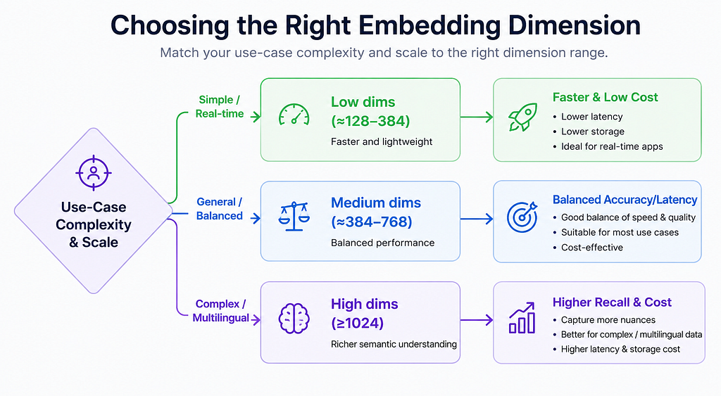
Short, Real-Time Queries (e.g. chat/autocomplete): Use low dimensions (~128–384). These applications demand <50 ms latencies, favoring minimal computation. For example, an internal wiki or FAQ search often works well with 256–384 dims. This also keeps memory and database costs low.
General Document Search (e.g. business FAQ, knowledge base): Moderate dimensions (~384–768) often suffice. Most typical enterprise documents (reports, product descriptions, tickets) are well-served in this range. The embeddings capture enough nuance without huge overhead. Industry practice bears this out: “for most applications, 384-dimensional embeddings provide sufficient semantic resolution”.
Long or Complex Documents: Long texts should be chunked, but each chunk’s embedding can use similar dims as above. However, if each chunk is very rich or multi-topic, consider higher dims (≥768) to encode more context. If queries themselves are long, chunk them or use models with extended context.
Multilingual Content: If searching in or across many languages, use higher dimensions (≥768) to capture cross-lingual semantics. Models like multilingual SBERT or XLM-R often have ≥768 dims. In practice, Particular notes that “models targeting multilingual use typically start at 768 dimensions minimum”.
Domain-Specific Technical/Scientific Data: Technical specs, legal documents, scientific papers or code often need more capacity. Guidelines suggest 1024–1536 dims for such use cases. For example, a company found 768 dims caused confusion across domains (legal vs marketing), and only 1536 dims fully separated them. Domain-specific fine-tuning can help, but having extra dimensions allows encoding subtle distinctions (modeling rare terms or detailed structures).
High-Recall vs Low-Resource: If your priority is maximum recall/accuracy (e.g. critical question-answering), you may choose higher dimensions as needed, accepting the cost. Conversely, for on-device or budget-constrained scenarios, lean on smaller dims. Distilled/smaller models (MiniLM, DistilBERT) at 256–384 dims often retain ~90–95% of accuracy at a fraction of the cost. For example, DistilBERT (768→384 dims) retains 95% of BERT’s performance with 60% less compute, enabling on-device or edge usage.
Batch (Offline) vs Online Search: In offline or batch analytics, you can afford higher dims since query latency is less critical. For interactive search or live APIs, favor lower dims to reduce QPS latency.

These are rules of thumb. Always test with your own data. In practice, most production systems fall in the 384–768 range, only jumping above 1024 dims for specialized needs.

Concrete Examples & Recommendations

The following table summarizes dimension ranges for different search tasks:

When resources are tight, quantization/PCA can help. For example, one could embed at 768 dims then apply PCA to 384 dims and store as int8 (16× size reduction). And remember: your users don’t care about dimension; they care about finding answers quickly. Optimize dimension for that.

Implementation Tips (Training, Compression, Evaluation)

Off-the-Shelf vs Training: Most practitioners use pretrained embeddings (SBERT, OpenAI, Cohere, etc.) with fixed dims. To change dimension, you can only train a new model or reduce dimensions post-hoc. Fine-tuning does not alter dimension; it just adjusts weights for your domain. If you need custom dimensions, you could train a small embedding model from scratch with your chosen architecture (not common) or adopt methods like Matryoshka (see below) that let you dynamically truncate embeddings.
Fine-Tuning: Always fine-tune (or instruction-tune) embeddings on domain-specific data if possible. Even a 384-dim model will perform better on your domain after fine-tuning. For example, a domain-specialized SBERT (384 dim) can outperform a generic 768-dim model on in-domain queries.
PCA (Principal Component Analysis): You can reduce dimensions after generating embeddings. For example, apply sklearn.decomposition.PCA to your corpus of vectors, choosing the top k components (say 256 from 768). This shrinks storage and speeds up search with a small accuracy hit. Many papers find that most variance lies in a few principal axes. After PCA, rebuild your index on the reduced vectors.

from sklearn.decomposition import PCA
pca = PCA(n_components=256).fit(doc_embeddings) 
docs_lowdim = pca.transform(doc_embeddings)
queries_lowdim = pca.transform(query_embeddings)

Product Quantization (PQ/OPQ): If you can’t reduce dimension, compress it. Faiss-style PQ splits vectors into subvectors and replaces each with a centroid index. This can compress e.g. 1024 dims into ~64-byte codes. Pinecone reports 97% memory reduction and >5× speedup. An IVF-PQ index (clustering + PQ) can boost search by 92× with no accuracy loss. Some vector DBs (Milvus, Faiss, Weaviate) support PQ/OPQ natively. The trade-off is some approximation error, so recall may dip if you compress too hard.
Quantization (Numerical): Lower numerical precision (float32→float16 or int8) cuts memory. Milvus notes float16 halves space. OPQ (Optimized Product Quantization) is a variant that rotates space before PQ for better accuracy. In practice, 8-bit quantization of embeddings typically loses only a few percent accuracy. E.g. combining PCA 1536→384 dims and then int8 quantization yields a 16× space reduction “with acceptable accuracy loss”.
Hybrid Sparse+Dense Retrieval: Dense embeddings can miss keyword-level signals (e.g. exact matches, numeric data). A common solution is to run a term-based model (BM25 or a sparse neural encoder) in parallel and combine results. This doesn’t directly relate to dimension choice, but it means you might get away with a smaller dense vector if lexical matching covers gaps.
Evaluation Metrics: Measure retrieval performance at each candidate dimension using standard IR metrics: Recall@k, Precision@k, Mean Reciprocal Rank (MRR), nDCG, etc. Recall is often key: it measures what fraction of truly relevant docs appear in the top k results. For example, you might track Recall@10 for a suite of queries as you vary dimensions. Also log query latency (P50/P95) and throughput under load. This tells you where dimension-scaling breaks your SLAs.
Benchmarking Code Example: The following pseudocode illustrates how one might benchmark recall at different dimensions:

import numpy as np
import faiss
from sklearn.metrics.pairwise import cosine_similarity

# Example data (replace with real embeddings)
doc_emb = np.random.randn(10000, 768).astype('float32')
query_emb = np.random.randn(100, 768).astype('float32')
true_ids = [...]  # list of ground-truth relevant doc IDs per query

for dim in [128, 256, 384, 512, 768]:
    # Truncate embeddings to first 'dim' components (or use PCA)
    docs_low = doc_emb[:, :dim]
    queries_low = query_emb[:, :dim]
    
    # Build a simple L2 index (could use HNSW or IVF+PQ for scale)
    index = faiss.IndexFlatL2(dim)
    index.add(docs_low)
    D, I = index.search(queries_low, k=10)  # top-10
    
    # Compute Recall@10
    hits = 0
    for qi, ans_ids in enumerate(true_ids):
        if any(i in ans_ids for i in I[qi]):
            hits += 1
    recall = hits / len(true_ids)
    print(f"Dim={dim}: Recall@10={recall:.2%}")

Checklist & Protocol:

Define Goals: Set target metrics (e.g. Recall@10 ≥ 90%, latency <50 ms).
Baseline: Pick a default dimension (e.g. 384) and measure performance on a representative dataset.
Scale Up Gradually: Increase to 512, 768, 1024… at each step measuring accuracy, latency, and cost. Look for the point of diminishing returns.
Calculate Costs: For each dimension, compute storage (Dim×#vectors×4 bytes) and latency (benchmark under realistic load). E.g. 1 M×1024 dims ≈ 4 GB, 3× storage vs 384 dims.
Factor in Constraints: If latency or memory budgets are tight, cap dimension. If certain queries fail at low dims, raise it.
Hybrid or Compression: If high dimension is needed but costs too high, consider PCA or PQ (dimensionality/precision reduction) and re-evaluate.
Monitor and Iterate: In production, track actual QPS and recall; adjust dimension (or indexing parameters) as data evolves.

Conclusion

Embedding dimension is a key design choice in semantic search, but there is no one-size-fits-all answer. The right dimension depends on your data complexity, accuracy requirements, and resource constraints. As the literature and our guidelines show, starting small and iterating is wise. In most cases 384–768 dimensions are “enough” — large enough to get good recall without blowing up storage or latency. Only go above 1024 dims when you have concrete evidence (from benchmarks on your domain) that accuracy gains justify the extra cost.

Amit Kumar is a Software Engineer specializing in backend architectures and AI-driven data pipelines.

If you enjoyed this article, feel free to follow for more insights on Java, Kafka, and the evolving AI landscape..

Choosing the Right Embedding Dimension for Semantic Search was originally published in Towards AI on Medium, where people are continuing the conversation by highlighting and responding to this story.

Back to Listing

credit: